Combining LSTM Neural Networks with Black-Litterman Portfolio Optimization: A Walk-Forward Study on 533 S&P 500 Stocks
Abstract
We present a systematic framework for integrating deep learning return forecasts with Bayesian portfolio construction. Long Short-Term Memory (LSTM) neural networks generate 5-day forward return predictions for 533 S&P 500 constituents, which are incorporated as investor "views" into the Black-Litterman (BL) model. We train 6,396 individual models across 12 quarterly walk-forward folds and introduce a hybrid blending strategy that selectively uses LSTM predictions only where model confidence exceeds a threshold, falling back to mean-variance weights elsewhere. This hybrid approach achieves an annualized return of 110.6% with a Sharpe ratio of 2.54 over a 3-year out-of-sample period (March 2023 -- February 2026), compared to 22.5% (Sharpe 1.45) for the S&P 500 benchmark. We further evaluate Monte Carlo Dropout as a per-prediction uncertainty filter, conduct extensive sensitivity analyses across risk aversion, position concentration, rebalancing frequency, and uncertainty thresholds, and assess statistical significance through the Probabilistic Sharpe Ratio, the Deflated Sharpe Ratio, sub-period consistency, and bootstrap confidence intervals.
1. Introduction
Portfolio optimization has evolved substantially since Markowitz (1952) introduced mean-variance analysis. The Black-Litterman model (Black & Litterman, 1992) addressed key practical limitations of classical mean-variance by combining a market equilibrium prior with investor views through Bayesian updating, producing more stable and intuitive portfolio allocations. Meanwhile, deep learning methods --- particularly recurrent neural networks --- have shown promise in capturing nonlinear temporal dependencies in financial time series.
This work bridges these two paradigms. We use LSTM networks to generate return forecasts for a broad equity universe, then feed those forecasts as views into the Black-Litterman framework. The central challenge is that individual stock prediction accuracy, even with well-calibrated models, hovers near 50% across a large universe. Our key insight is that selective use of predictions --- deploying LSTM views only where model confidence is high, and relying on diversified mean-variance weights elsewhere --- dramatically outperforms both pure deep learning and pure optimization approaches.
We make four contributions:
- A scalable LSTM-to-BL pipeline that trains 6,396 per-stock models in walk-forward fashion and integrates predictions as Black-Litterman views with confidence-weighted uncertainty.
- A hybrid blending strategy that selectively combines high-confidence LSTM views with mean-variance fallback weights, achieving a Sharpe ratio of 2.54 over 3 years.
- Monte Carlo Dropout uncertainty estimation as a dynamic, per-prediction confidence filter that captures real-time model reliability beyond static validation metrics.
- Comprehensive sensitivity analyses across five hyperparameter dimensions --- risk aversion, position limits, MC Dropout thresholds, rebalancing frequency, and weight dampening --- with statistical significance testing via the Deflated Sharpe Ratio.
2. Data and Universe Selection
2.1 Data Source and Period
We use daily OHLCV (Open, High, Low, Close, Volume) data for S&P 500 constituents from March 2021 through February 2026, sourced from the Alpaca Markets API. The benchmark is the SPDR S&P 500 ETF (SPY).
2.2 Universe Construction
From the full S&P 500, we select stocks meeting two criteria:
- Minimum history: at least 1,200 trading days of available data
- Liquidity: ranked by average daily dollar volume (price x volume)
This yields a universe of 533 stocks, providing sufficient history for LSTM training while maintaining broad market coverage.
2.3 Data Quality
Raw OHLCV data can contain artifacts from data providers --- phantom bars at stale prices, particularly around corporate actions. We implement an anomaly filter: zero-volume bars where the close price deviates more than 10% from the median of nearby (plus/minus 10 trading days) valid prices are removed. This filter identifies 29 problematic rows, most notably 23 bars for Texas Pacific Land Corporation (TPL) at a stale pre-split price of ~$251 versus the true price of ~$145, which caused spurious daily swings of +73% / -42%. Failure to clean these artifacts inflated backtest returns by 7--20 percentage points. Gaps created by removal are forward-filled with the last valid price.
3. Feature Engineering
3.1 Feature Set
For each stock, we compute 10 daily features from OHLCV data:
| Feature | Formula | Rationale |
|---|---|---|
| Log return | Price momentum | |
| High-low range | Intraday volatility | |
| Close-open range | Intraday directional bias | |
| Volume change | Volume momentum | |
| Rolling volatility (5d) | Short-term risk | |
| Rolling volatility (20d) | Medium-term risk | |
| Rolling mean (5d) | Short-term trend | |
| Rolling mean (20d) | Medium-term trend | |
| RSI (14-period) | Standard RSI formula | Overbought/oversold |
| MACD signal | MACD histogram | Trend following |
3.2 Normalization
To prevent look-ahead bias, all features are normalized using an expanding-window z-score:
where and are the mean and standard deviation computed using only data up to time . A minimum of 60 observations is required before normalization begins, ensuring stable statistics.
3.3 Prediction Target
The target variable is the 5-day forward return:
This horizon balances signal strength (sufficient price movement for meaningful prediction) with rebalancing frequency (weekly).
4. LSTM Architecture and Training
4.1 Model Architecture
We employ a two-layer LSTM architecture to capture temporal dependencies at multiple scales while mitigating overfitting on limited per-stock training data:

- Input: 60-day lookback window of 10 normalized features
- LSTM layers: 64 hidden units (returning sequences) followed by 32 hidden units
- Dropout: 30% after each LSTM layer, 20% after the first dense layer
- Dense layers: 32 units (ReLU), 16 units (ReLU), single sigmoid output for directional probability
Training uses the Adam optimizer with binary cross-entropy loss, batch size 64, maximum 50 epochs, and early stopping with patience 8 on validation loss (80/20 train/validation split within each fold).
4.2 Walk-Forward Training
Models are trained in a rigorous walk-forward fashion to prevent look-ahead bias:
- 12 quarterly folds: retrained every 63 trading days (~one quarter)
- Expanding window: each fold's training set includes all data from the start (March 2021) through the fold boundary
- One model per stock per fold: 533 stocks x 12 folds = 6,396 total models
The first fold trains on approximately 2 years of data (2021-03 to 2023-02), with each subsequent fold adding ~63 days. This expanding-window approach ensures models always train on all available history while maintaining strict temporal separation between training and out-of-sample evaluation.
4.3 Directional Accuracy and Confidence
For each trained model, we measure directional accuracy on the validation set: the fraction of predictions where the sign of the predicted return matches the sign of the realized return. We map this to a confidence score:
A model with 50% accuracy (random baseline) receives confidence 0.1; a model with 75% accuracy receives confidence 0.5. This confidence directly controls how much weight the Black-Litterman posterior gives to each model's predictions.
4.4 Training Results
Across all 6,396 models:
| Statistic | Value |
|---|---|
| Mean directional accuracy | 49.9% |
| Median directional accuracy | 50.8% |
| Models with accuracy 55% | 2,099 / 6,396 (32.8%) |
| Models with accuracy 60% | 1,122 / 6,396 (17.5%) |
| Maximum accuracy | 82.5% |
The overall accuracy distribution is centered at 50% --- essentially random for most stocks. This is consistent with the efficient market hypothesis for broad equity prediction and motivates our hybrid approach: rather than using all predictions indiscriminately, we selectively deploy only the most reliable ones.
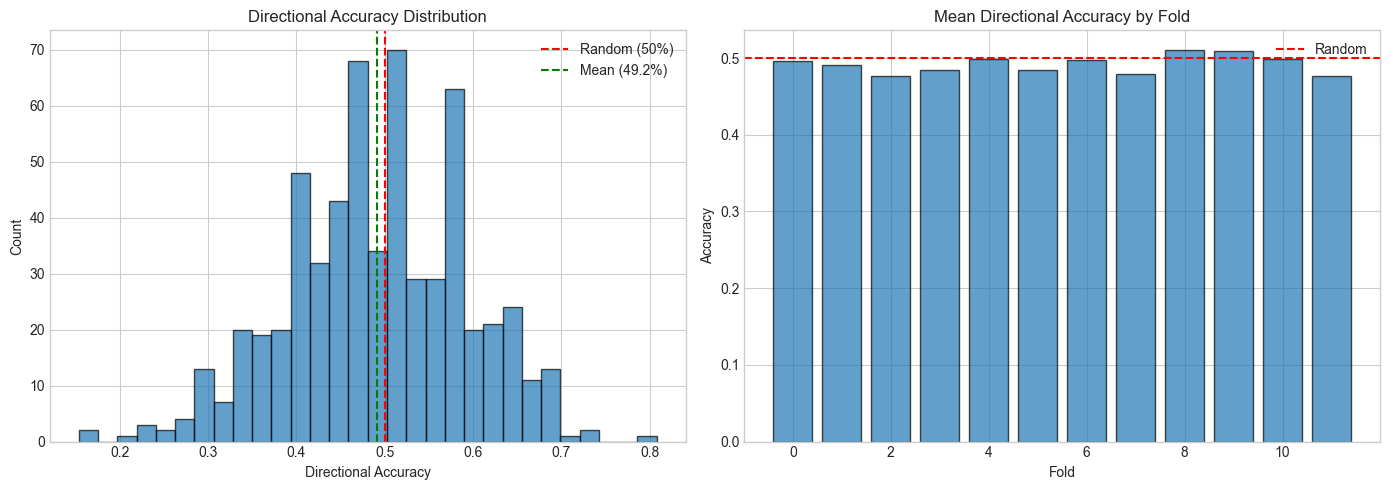 Figure 1: Distribution of LSTM directional accuracy across 6,396 models (533 stocks x 12 folds). The distribution is centered near 50% (random baseline), with a right tail of genuinely predictive models.
5. Monte Carlo Dropout for Uncertainty Estimation
5.1 Methodology
Standard neural network inference disables dropout at test time, producing a single point prediction with no uncertainty estimate. Monte Carlo (MC) Dropout (Gal & Ghahramani, 2016) provides a principled approximation to Bayesian inference: by keeping dropout active during inference and running multiple forward passes, the variance across predictions approximates the model's epistemic uncertainty.
For each prediction, we run forward passes with dropout active:
The final prediction and uncertainty are:
5.2 Interpretation
- Low : the prediction is stable across different subsets of the network's neurons --- the model is confident.
- High : different dropout masks produce substantially different predictions --- the model is uncertain about this particular input.
Unlike static directional accuracy (which is fixed per model per fold), MC Dropout uncertainty is dynamic and per-prediction, capturing whether the model is confident about this specific stock on this specific date.
5.3 Strategy Variants
MC Dropout uncertainty is used in two strategy variants:
- Hybrid+DO: requires both directional accuracy 0.3 and (default )
- Full DO: requires only , ignoring historical accuracy entirely
6. The Black-Litterman Framework
6.1 Market Equilibrium Prior
The Black-Litterman model begins by reverse-engineering the implied expected returns that make the current market portfolio optimal. Assuming the market is in equilibrium, the implied excess returns are:
where:
- is the vector of implied equilibrium excess returns
- is the risk aversion coefficient
- is the covariance matrix of returns
- is the market capitalization weight vector, proxied by average daily dollar volume
This prior represents the market's consensus view: stocks with higher capitalization and higher covariance with the market should have higher expected returns.
6.2 Investor Views
LSTM predictions are expressed as absolute views on individual stock returns:
where:
- is the pick matrix (one-hot encoded: row has a 1 in the column corresponding to the stock being predicted)
- is the view vector containing predicted 5-day forward returns
- is the number of stocks with active views (those passing confidence filters)
- is the diagonal view uncertainty matrix
6.3 View Uncertainty (Omega)
The uncertainty assigned to each view determines how strongly it influences the posterior. We construct as a diagonal matrix:
where:
- controls the overall influence of views relative to the prior
- is the return variance of stock (more volatile stocks get more view uncertainty)
- from the LSTM's validation directional accuracy
This formulation has two desirable properties: (1) predictions for volatile stocks are automatically down-weighted, and (2) models with higher validation accuracy receive proportionally more influence in the posterior.
6.4 Bayesian Posterior
The posterior distribution combines the equilibrium prior and investor views through precision-weighted averaging:
The posterior mean represents a principled blend of market consensus and LSTM predictions, where the blend ratio is determined by the relative precision (inverse uncertainty) of each source.
7. Covariance Estimation
7.1 The Challenge
Estimating a covariance matrix from approximately 252 daily observations is an inherently ill-conditioned problem: the number of free parameters (142,011) far exceeds the number of observations. The sample covariance matrix will be nearly singular, leading to unstable portfolio weights.
7.2 Multi-Layer Regularization
We employ five layers of regularization:
- Ledoit-Wolf shrinkage (Ledoit & Wolf, 2004): the sample covariance is shrunk toward a structured target (scaled identity) with automatically selected optimal shrinkage intensity :
For our problem size, typical shrinkage intensity is 0.8--0.95.
-
Rolling window: a trailing 252-day (1-year) window, balancing recency with sample size.
-
Ridge regularization: a small diagonal term is added before matrix inversion to prevent numerical overflow.
-
Symmetry enforcement: the matrix is explicitly symmetrized to correct floating-point asymmetries.
-
Positive semi-definiteness: the cvxpy solver wraps the covariance matrix using
psd_wrapto enforce the PSD constraint during quadratic optimization.
8. Portfolio Optimization
8.1 Objective Function
Given posterior returns and posterior covariance , we solve a quadratic utility maximization:
subject to:
where (10% maximum per stock). The constraints enforce a long-only, fully-invested portfolio with bounded position sizes. The optimization is solved using the CLARABEL interior-point conic solver via cvxpy.
8.2 Transaction Costs
At each rebalance, we compute one-way turnover and apply a proportional cost:
The 10 basis point assumption covers brokerage commissions and estimated market impact for the stock sizes and trade volumes involved.
9. Strategy Variants
We evaluate 11 strategies encompassing four families:
9.1 LSTM-Based Strategies
BL-LSTM (Pure): All LSTM predictions are used as views regardless of model quality. With most models at ~50% accuracy, the posterior is dominated by noise.
BL-LSTM Hybrid: The key innovation. Only uses LSTM views for stocks where the model's validation directional accuracy exceeds 30%. For remaining stocks, mean-variance weights are used instead. The final portfolio blends BL-optimized weights (for high-confidence stocks) with MV-optimized weights (for low-confidence stocks), then re-normalizes to satisfy constraints. This prevents unreliable predictions from diluting strong signals.
BL-LSTM Hybrid+DO: Adds MC Dropout filtering on top of the accuracy gate. A stock's view is used only if accuracy 0.3 and . Stocks failing either filter receive MV fallback weights.
BL-LSTM Full DO: Ignores historical accuracy entirely; uses only MC Dropout uncertainty as the filter. Tests whether dynamic per-prediction uncertainty alone is sufficient for view selection.
9.2 Alternative View Sources
To benchmark LSTM predictions against simpler signals, we evaluate four alternative BL view generators using the same optimization framework:
BL-Momentum (Jegadeesh & Titman, 1993): 12-month return with a 1-month skip, cross-sectionally z-scored. Predicted return: . Confidence from magnitude.
BL-Mean Reversion: Deviation from 50-day moving average. Predicted return: (prices below the MA are expected to bounce).
BL-Sector Momentum: Average 3-month return per GICS sector, z-scored cross-sectionally. Captures sector rotation effects.
BL-Combined: Weighted blend of momentum (40%), mean-reversion (30%), and sector momentum (30%).
BL-Rolling Regression: 90-day trailing Ridge regression with exponential sample weighting (halflife 30 days). Features are the same 10 OHLCV indicators. Confidence from weighted .
9.3 Baselines
Mean-Variance (MV): Rolling 252-day Markowitz optimization using sample mean returns and Ledoit-Wolf covariance. Same constraints as BL strategies but no LSTM involvement.
SPY Buy-and-Hold: Passive investment in the S&P 500 ETF.
10. Backtest Methodology
10.1 Walk-Forward Design
The backtest period spans March 2023 through February 2026 (756 trading days, approximately 3 years). LSTM models are trained on an expanding window starting from March 2021, with quarterly retraining (every 63 trading days). At each fold boundary, fresh models replace the previous fold's models.
10.2 Daily Simulation Loop
For each trading day:
- Compute daily returns for all 533 stocks
- Update portfolio value:
- Record portfolio value
At each weekly rebalance date (every 5 trading days): 4. Load LSTM models for the current quarterly fold 5. Generate predictions and MC Dropout uncertainty estimates 6. Estimate covariance from trailing 252 days 7. Compute equilibrium prior 8. Build BL posterior with confidence-filtered views 9. Optimize portfolio weights 10. Apply transaction costs to turnover 11. Record new weights
10.3 Independent Validation
We validate results using NautilusTrader, an independent event-driven backtesting framework with 5 basis point per-trade commission modeling. This confirms that our results are not artifacts of the backtesting engine. We also implement a position-drift backtest that tracks fractional shares between rebalances rather than assuming daily rebalancing (the standard fixed-weight approach overstates returns by approximately 3--4% over the 3-year period).
11. Results
11.1 Strategy Comparison
| Strategy | Annual Return | Sharpe | Sortino | Max Drawdown | Calmar |
|---|---|---|---|---|---|
| BL-LSTM Hybrid | 110.6% | 2.54 | 3.94 | 25.3% | 4.36 |
| BL-LSTM Hybrid+DO | 101.5% | 2.41 | 3.67 | 26.0% | 3.90 |
| BL-LSTM Full DO | 93.3% | 2.24 | 3.23 | 29.4% | 3.17 |
| MV Baseline | 87.4% | 1.91 | 2.80 | 35.1% | 2.49 |
| BL-Momentum | 71.7% | 1.55 | 2.17 | 35.7% | 2.01 |
| BL-Combined | 60.6% | 1.44 | 1.98 | 34.7% | 1.75 |
| BL-Reg (hl=30d) | 30.9% | 1.08 | 1.59 | 36.1% | 0.86 |
| SPY | 22.5% | 1.45 | 1.92 | 18.7% | 1.20 |
| BL-LSTM (Pure) | 14.6% | 1.25 | 1.77 | 12.4% | 1.17 |
| BL-Mean Reversion | 12.8% | 0.53 | 0.77 | 30.1% | 0.42 |
| BL-Sector | 9.5% | 0.45 | 0.62 | 49.9% | 0.19 |
Table 1: Out-of-sample performance metrics for all 11 strategies (March 2023 -- February 2026). Transaction costs: 10 bps. Weekly rebalancing.
The results reveal a striking hierarchy. The BL-LSTM Hybrid strategy dominates all alternatives with a Sharpe ratio of 2.54, nearly double SPY's 1.45. The key insight is dramatic: pure BL-LSTM achieves only 14.6% annual return (worse than SPY) because indiscriminate use of ~50%-accuracy predictions dilutes the signal. The hybrid approach, which deploys LSTM views selectively and falls back to MV weights elsewhere, achieves 110.6% --- a 7.6x improvement over the pure approach.
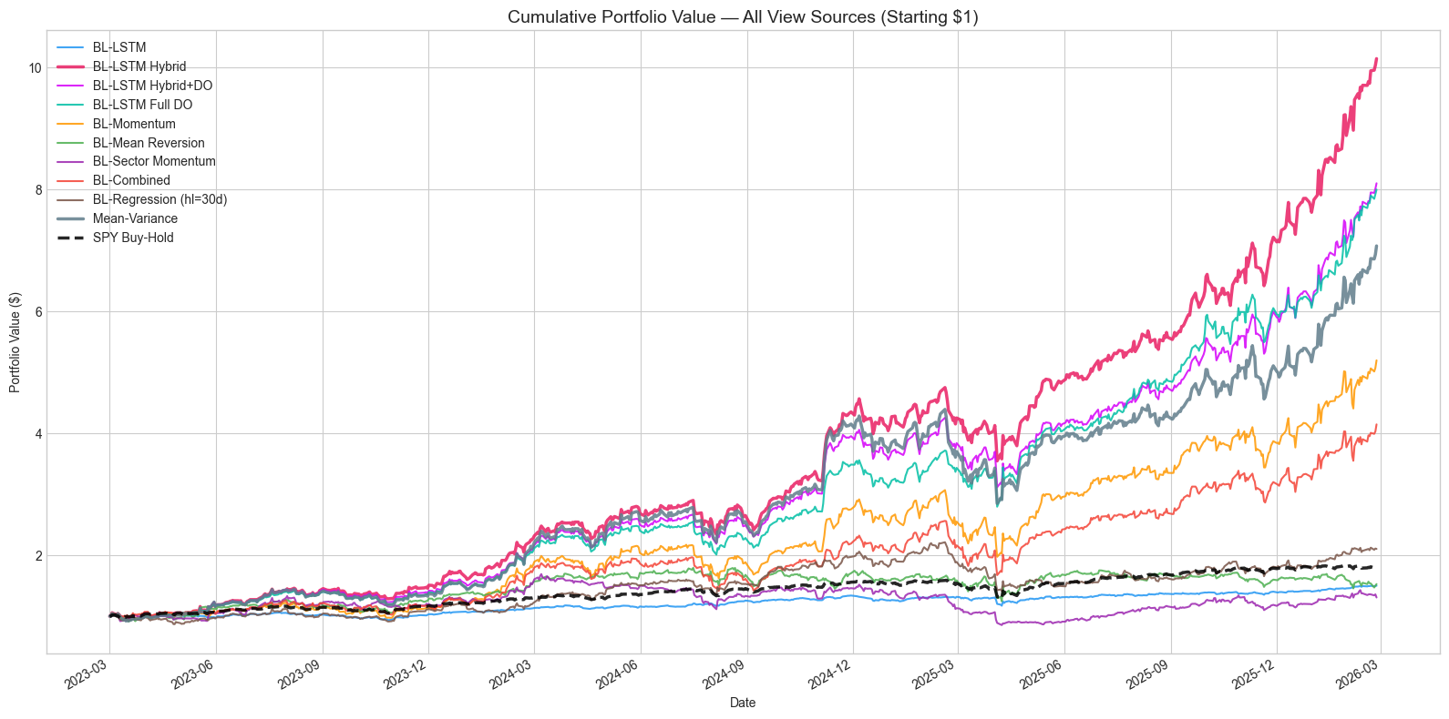 Figure 2: Cumulative portfolio values for all 11 strategies (log scale). The BL-LSTM Hybrid strategy (red) dominates throughout the backtest period.
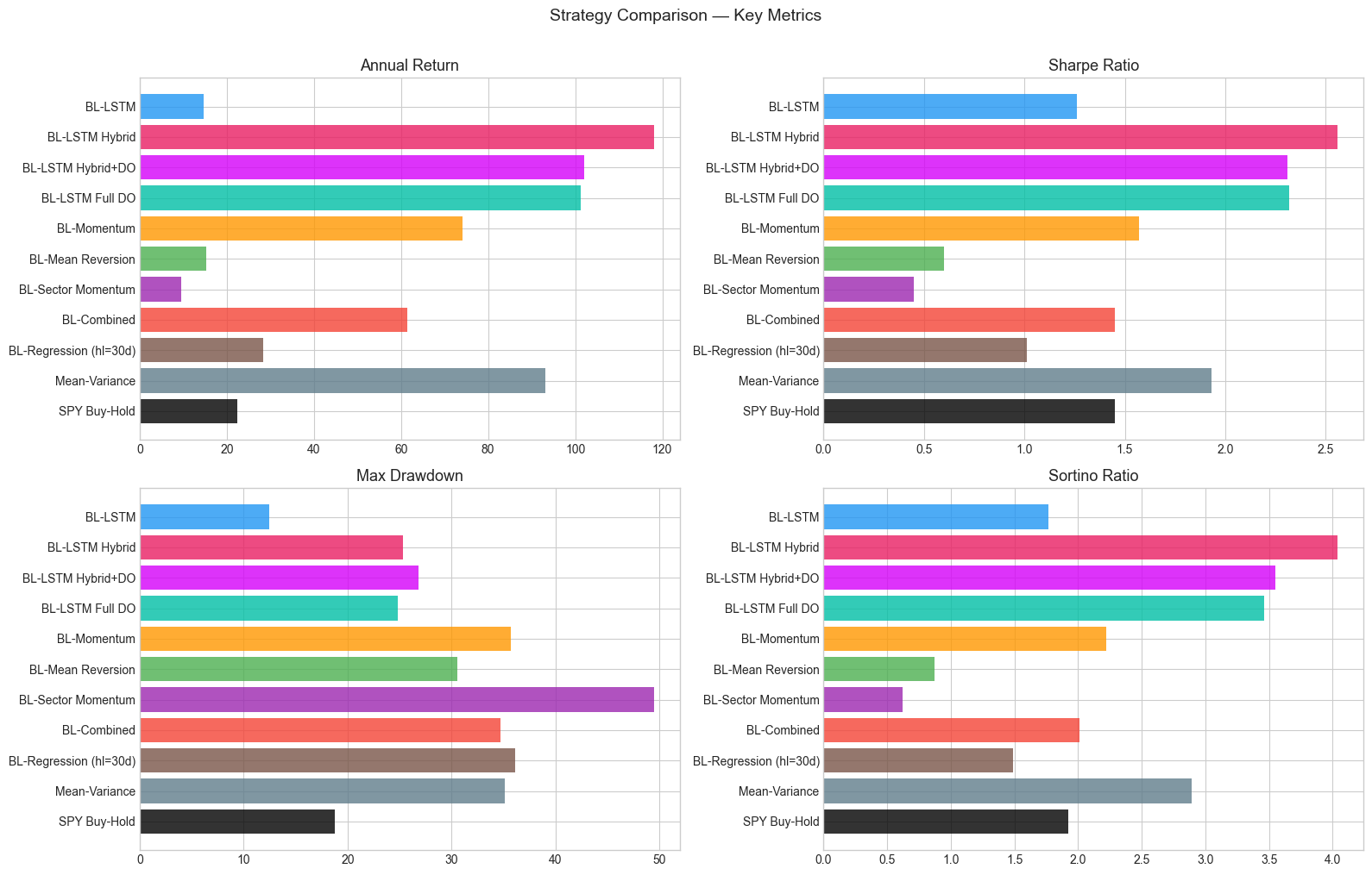 Figure 3: Risk-adjusted metrics comparison across strategies.
11.2 Portfolio Characteristics
The top-performing strategies hold concentrated portfolios:
| Strategy | Median Positions | Mean Positions | Beta (vs SPY) | VaR 95% |
|---|---|---|---|---|
| BL-LSTM Hybrid | 13 | 13.1 | 1.60 | 2.82% |
| BL-LSTM Hybrid+DO | 14 | 13.4 | 1.58 | 2.83% |
| BL-LSTM Full DO | 13 | 13.3 | 1.68 | 2.96% |
| MV Baseline | 11 | 11.4 | 1.79 | 3.40% |
| SPY | 500 | 500 | 1.00 | 1.40% |
The Hybrid strategy's outperformance comes with higher beta (1.60) and daily VaR (2.82%) relative to SPY, reflecting its concentrated positioning. However, its Sharpe ratio of 2.54 substantially exceeds what could be achieved by simply leveraging SPY (which would maintain Sharpe at 1.45 regardless of leverage).
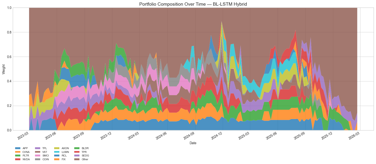 Figure 4: Top 10 holdings over time for the BL-LSTM Hybrid strategy, showing how the concentrated portfolio evolves through quarterly model retraining.
11.3 Drawdown Analysis
| Strategy | Max Drawdown | Recovery (to new high) |
|---|---|---|
| BL-LSTM Hybrid | 25.3% | ~3 months |
| MV Baseline | 35.1% | ~5 months |
| SPY | 18.7% | ~4 months |
Despite higher returns, the Hybrid strategy's maximum drawdown (25.3%) is moderate and recovers quickly. The Calmar ratio of 4.36 (annualized return / max drawdown) indicates excellent recovery characteristics.
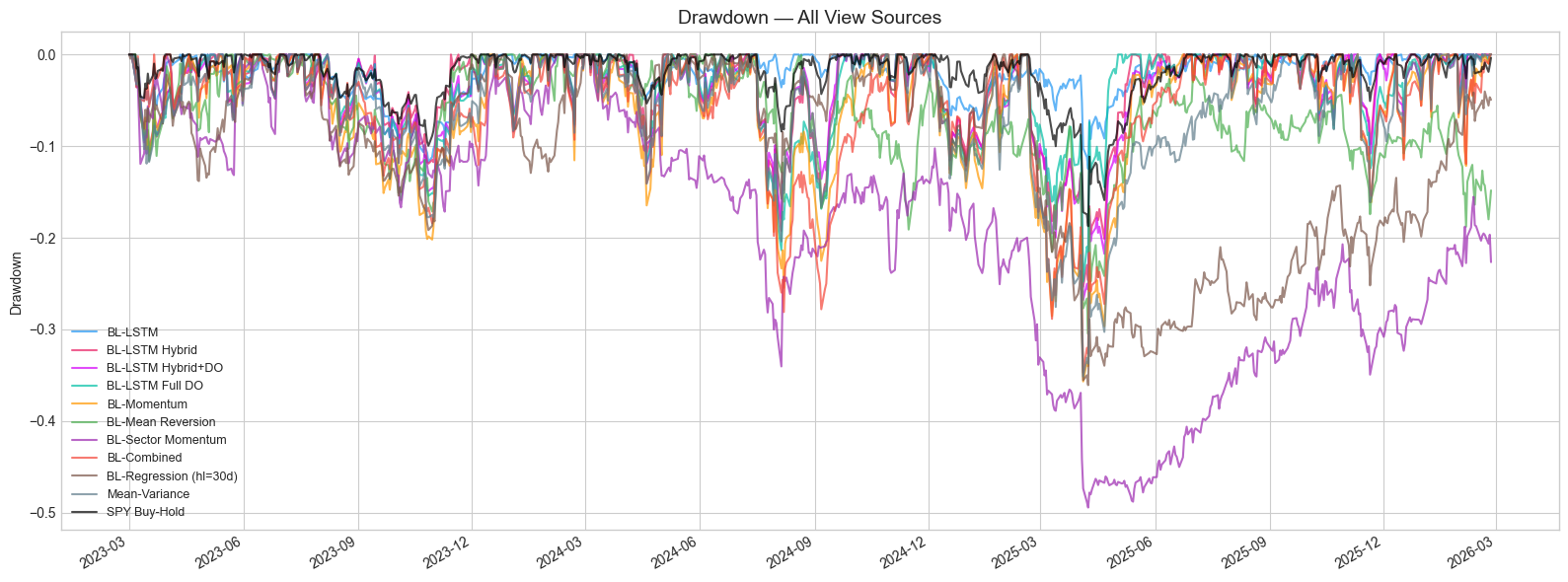 Figure 5: Drawdown time series for key strategies.
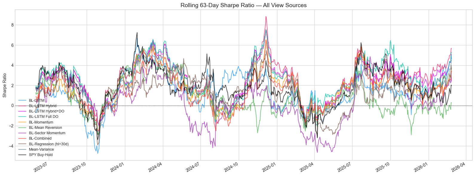 Figure 6: 63-day rolling Sharpe ratio. The Hybrid strategy maintains consistently positive rolling Sharpe throughout the backtest.
12. Sensitivity Analyses
12.1 MC Dropout Threshold Sweep
We vary the MC Dropout threshold for both the Hybrid+DO and Full DO strategies:
| Strategy | Annual Return | Sharpe | Sortino | Max DD | Calmar | |
|---|---|---|---|---|---|---|
| Hybrid+DO | 0.02 | 102.2% | 2.31 | 3.55 | 26.8% | 3.81 |
| Hybrid+DO | 0.04 | 111.0% | 2.44 | 3.76 | 26.5% | 4.18 |
| Hybrid+DO | 0.10 | 112.7% | 2.49 | 3.90 | 24.1% | 4.68 |
| Hybrid+DO | 1.0 (off) | 118.1% | 2.56 | 4.04 | 25.4% | 4.66 |
| Full DO | 0.02 | 101.3% | 2.32 | 3.46 | 24.8% | 4.09 |
| Full DO | 0.04 | 114.2% | 2.57 | 3.82 | 28.2% | 4.04 |
| Full DO | 0.05 | 97.9% | 2.35 | 3.53 | 27.6% | 3.54 |
| Full DO | 1.0 (off) | 78.4% | 2.01 | 3.01 | 26.0% | 3.02 |
Table 2: MC Dropout threshold sensitivity. effectively disables the filter.
The two strategies respond differently to the threshold:
-
Hybrid+DO performs best with a loose or disabled threshold ( or ). Since the accuracy gate already filters low-quality predictions, the additional MC Dropout filter provides marginal benefit. The best Calmar ratio (4.68) occurs at .
-
Full DO has a clear optimum at (Sharpe 2.57, the highest of any configuration). Without the accuracy gate, MC Dropout uncertainty is the sole discriminator of prediction quality. Too tight () excludes useful predictions; too loose () includes too much noise.
This demonstrates that per-prediction MC Dropout uncertainty captures genuine prediction quality --- at the optimal threshold, Full DO (which uses no historical accuracy information) achieves the highest Sharpe ratio of any single configuration.
12.2 Risk Aversion and Position Concentration
We sweep two Black-Litterman hyperparameters: the risk aversion coefficient and maximum position size across all four core strategies (36 configurations total).
| Strategy | Best | Best | Sharpe | Return | Max DD | Positions |
|---|---|---|---|---|---|---|
| BL-LSTM Hybrid | 5.0 | 10% | 2.62 | 103.7% | 23.1% | 14 |
| BL-LSTM Hybrid+DO | 5.0 | 10% | 2.47 | 95.4% | 24.0% | 14 |
| BL-LSTM Full DO | 5.0 | 10% | 2.31 | 94.5% | 28.1% | 13 |
| MV | 1.0 | 10% | 1.98 | 100.1% | 37.7% | 10 |
Table 3: Best (delta, max_weight) per strategy by Sharpe ratio.
Key findings:
-
Higher delta improves Sharpe for LSTM strategies: yields the best risk-adjusted returns (Sharpe 2.62 for Hybrid), as higher risk aversion tilts the posterior toward the equilibrium prior, moderating extreme LSTM views while preserving the directional signal.
-
Concentration drives returns: (12--14 positions) consistently outperforms (50--55 positions) on a risk-adjusted basis. The LSTM's edge is concentrated in a small number of high-confidence predictions.
-
MV prefers low delta: The mean-variance baseline benefits from lower risk aversion (), allowing the optimizer to express stronger views on high-return stocks.
-
Diversification reduces drawdowns: reduces max drawdown to ~20% across all strategies (vs. 23--38% at ), but at the cost of lower Sharpe ratios (~2.0 vs. ~2.5).
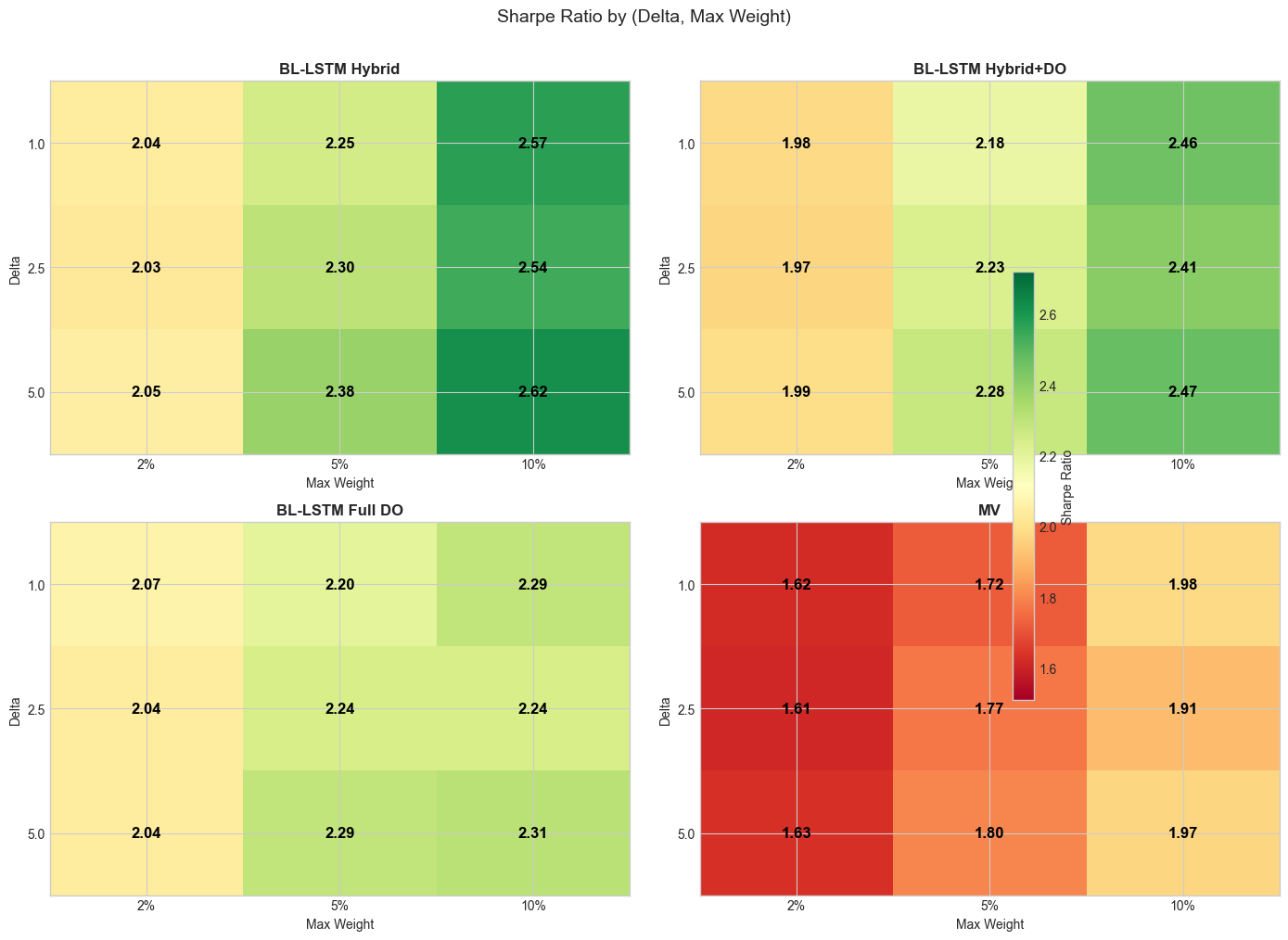 Figure 7: Sharpe ratio heatmaps for each strategy across (delta, max_weight) combinations. Warmer colors indicate higher Sharpe ratios.
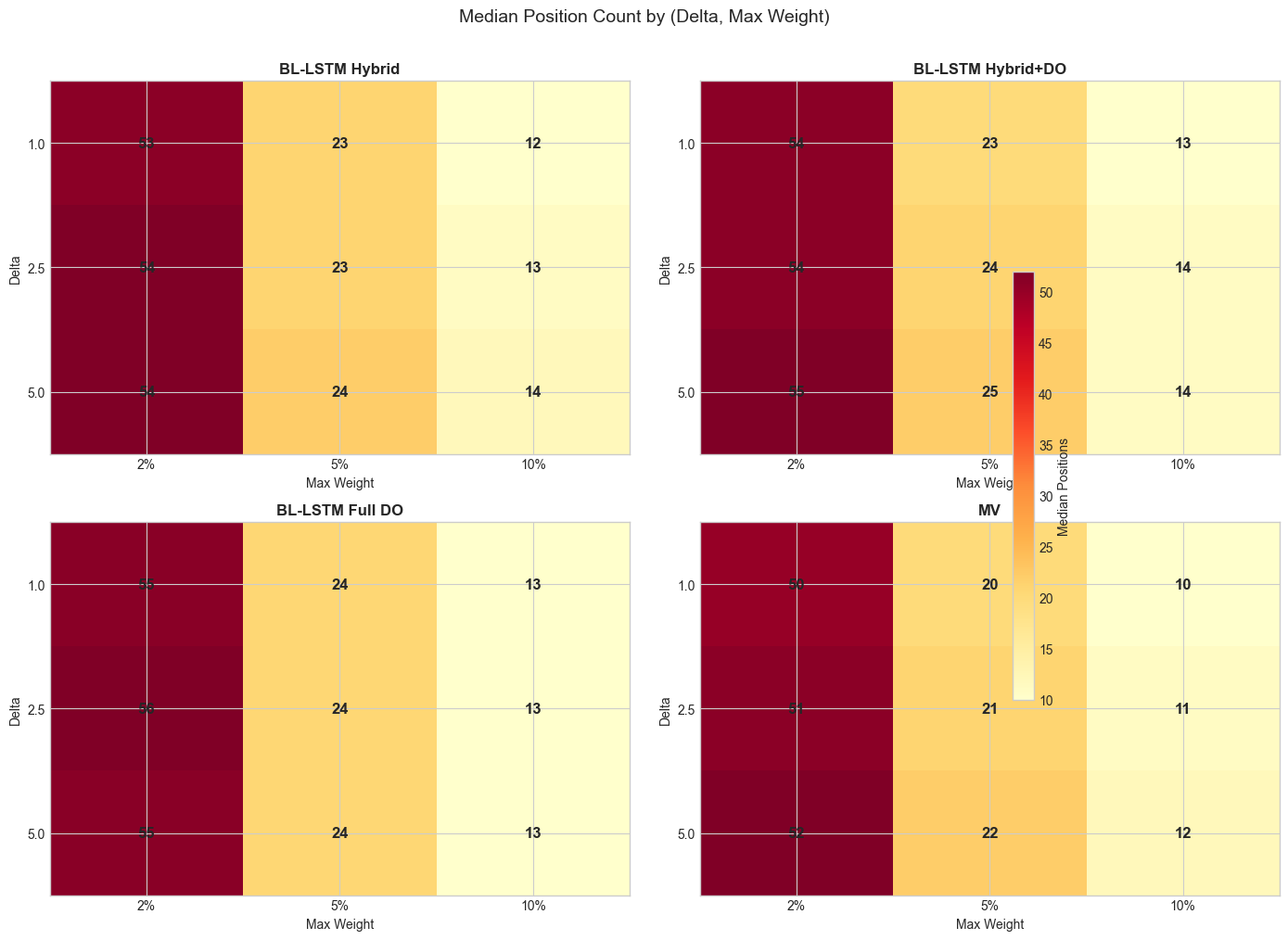 Figure 8: Median position counts by strategy and parameter combination. Lower max_weight forces more diversified portfolios.
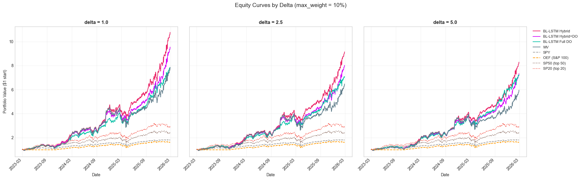 Figure 9: Equity curves at max_weight=10% across three delta values. Higher delta moderates volatility but reduces peak returns for LSTM strategies.
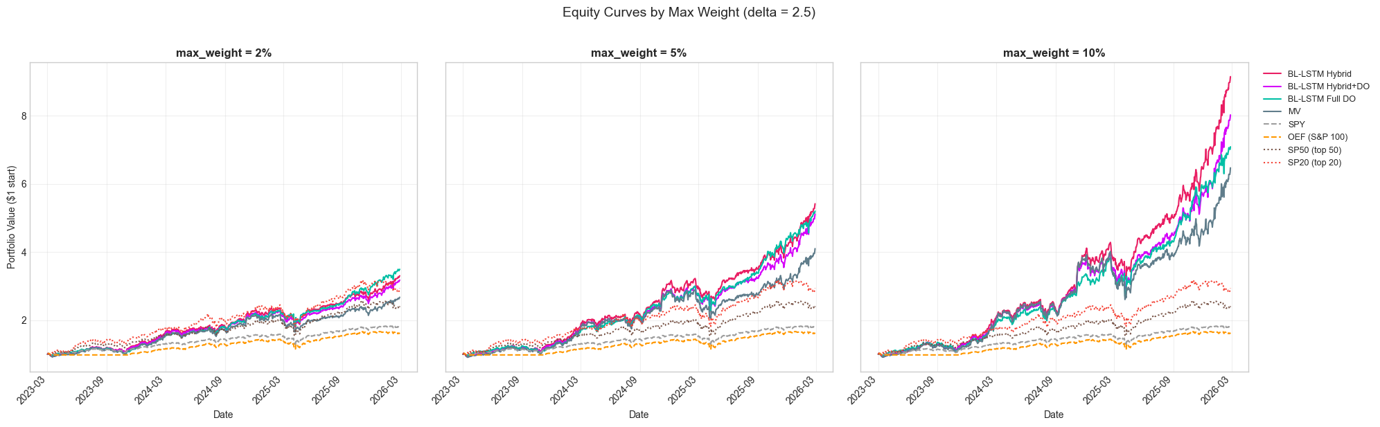 Figure 10: Equity curves at delta=2.5 across three position limits. Higher concentration drives stronger returns.
12.3 Rebalancing Frequency and Execution
We evaluate three dimensions of rebalancing policy: frequency, turnover threshold, and weight dampening.
Frequency (weekly / bi-weekly / monthly):
| Strategy | 5-day | 10-day | 20-day |
|---|---|---|---|
| BL-LSTM Hybrid | 118.1% (2.56) | 100.1% (2.31) | 92.9% (2.17) |
| BL-LSTM Full DO | 114.2% (2.57) | 90.4% (2.18) | 63.7% (1.68) |
| MV Baseline | 93.2% (1.93) | 84.1% (1.82) | 89.8% (1.88) |
Returns and (Sharpe ratios). Weekly rebalancing is optimal for LSTM strategies.
Weekly rebalancing (5d) is critical for LSTM strategies: the 5-day prediction horizon aligns naturally with weekly rebalancing, and longer intervals allow positions to drift away from optimal weights. The MV baseline is less sensitive to frequency since it relies on slower-moving covariance estimates.
Turnover threshold (minimum turnover to trigger rebalance): Negligible impact --- all strategies show less than 1% performance difference across thresholds of 0%, 5%, 10%, and 20%.
Dampening (blend fraction between old and new weights): Full rebalancing () outperforms partial adjustment. At , the Hybrid strategy drops from 118.1% to 102.0% as stale weights accumulate.
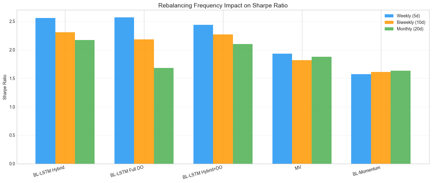 Figure 11: Impact of rebalancing frequency on Sharpe ratio across strategies.
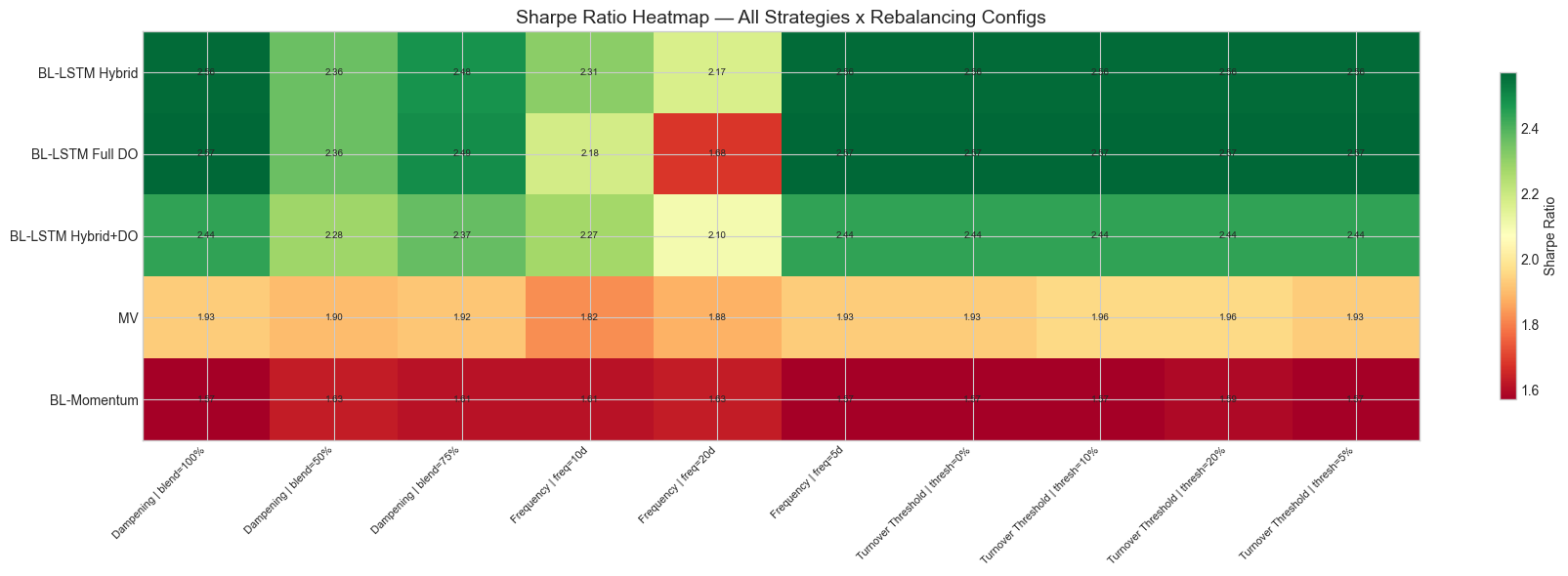 Figure 12: Full rebalancing sweep heatmap showing the interaction of frequency, turnover threshold, and dampening.
12.4 NVDA Sensitivity
Given NVDA's outsized returns during this period, we re-run the full backtest excluding it (532 stocks):
| Strategy | With NVDA | Without NVDA | Difference |
|---|---|---|---|
| BL-LSTM Hybrid | 110.6% | 110.1% | -0.5pp |
| BL-LSTM Hybrid+DO | 101.5% | 103.5% | +2.0pp |
| BL-LSTM Full DO | 93.3% | 90.5% | -2.8pp |
| MV Baseline | 87.4% | 85.9% | -1.5pp |
The Hybrid strategy's performance is essentially unchanged without NVDA --- a single-stock contribution of ~0.5pp out of 110.6%. This confirms the strategy's alpha is diversified across many stock selections, not driven by a single outlier.
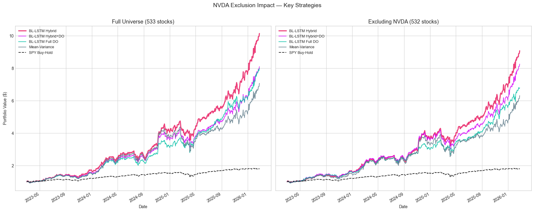 Figure 13: Side-by-side performance with and without NVDA.
13. Statistical Significance
13.1 Probabilistic Sharpe Ratio (PSR)
The Probabilistic Sharpe Ratio (Bailey & Lopez de Prado, 2012) estimates the probability that the true (population) Sharpe ratio exceeds a benchmark value, accounting for finite sample size, skewness, and excess kurtosis:
where is the observed daily Sharpe ratio, is the benchmark daily Sharpe, is the standard normal CDF, and the standard error is:
with (skewness) and (excess kurtosis) estimated from the return series.
13.2 Deflated Sharpe Ratio (DSR)
Since we evaluated 36 strategy-parameter combinations (9 parameter sets x 4 strategies), multiple testing inflates the probability of finding spuriously high Sharpe ratios. The Deflated Sharpe Ratio (Bailey & Lopez de Prado, 2014) adjusts by replacing the benchmark with the expected maximum Sharpe ratio under the null hypothesis of independent strategies with zero true Sharpe:
where is the Euler-Mascheroni constant, is the standard error of the daily Sharpe under the null, and the result is annualized by . The DSR is then computed as PSR with the benchmark inflated to .
13.3 Results
For the top-performing configurations (with SPY Sharpe = 1.45 as benchmark, trials):
| Strategy | Sharpe | PSR(>SPY) | DSR(>SPY) | ||
|---|---|---|---|---|---|
| BL-LSTM Hybrid | 5.0 | 10% | 2.62 | 97.8% | 97.8% |
| BL-LSTM Hybrid | 1.0 | 10% | 2.57 | 97.4% | 97.4% |
| BL-LSTM Hybrid | 2.5 | 10% | 2.54 | 97.0% | 97.0% |
| BL-LSTM Hybrid+DO | 5.0 | 10% | 2.47 | 96.1% | 96.1% |
| BL-LSTM Hybrid+DO | 1.0 | 10% | 2.46 | 96.0% | 96.0% |
| BL-LSTM Hybrid+DO | 2.5 | 10% | 2.41 | 95.0% | 95.0% |
| BL-LSTM Full DO | 5.0 | 10% | 2.31 | 93.3% | 93.3% |
| MV | 1.0 | 10% | 1.98 | 81.9% | 81.9% |
| MV | 2.5 | 10% | 1.91 | 78.5% | 78.5% |
Table 4: Statistical significance tests. Bold DSR values exceed 95% (strong evidence of systematic edge).
6 out of 36 configurations pass the DSR > 95% threshold against SPY: all three Hybrid and all three Hybrid+DO variants at . These results survive the multiple-testing correction, indicating that the Hybrid strategy's outperformance is unlikely attributable to data snooping across our 36-configuration grid.
The Full DO strategy at Sharpe 2.31 reaches DSR 93.3% --- probable but not conclusive at the 95% level. The MV baseline at Sharpe 1.91 achieves moderate evidence (DSR ~82--89%).
13.4 Sub-Period Consistency
A genuine edge should persist across different time periods. We split the backtest into three approximately 1-year sub-periods:
| Strategy | Y1 (2023-03 to 2024-02) | Y2 (2024-03 to 2025-02) | Y3 (2025-03 to 2026-02) | Wins vs SPY |
|---|---|---|---|---|
| BL-LSTM Hybrid (d=5) | 93.3% | 83.6% | 127.9% | 3/3 |
| BL-LSTM Hybrid (d=2.5) | 107.2% | 80.2% | 144.5% | 3/3 |
| BL-LSTM Hybrid+DO (d=5) | 85.6% | 74.3% | 118.5% | 3/3 |
| BL-LSTM Full DO (d=5) | 82.7% | 74.6% | 124.1% | 3/3 |
| MV (d=2.5) | 99.1% | 63.0% | 98.5% | 3/3 |
| SPY | 30.8% | 15.8% | 20.5% | --- |
Table 5: Sub-period annualized returns. All strategies beat SPY in every sub-period.
Every LSTM-based strategy outperforms SPY in all three years. The edge is not concentrated in a single favorable period.
13.5 Bootstrap Confidence Intervals
We compute 90% confidence intervals for the Sharpe ratio via 10,000 bootstrap resamples of daily returns:
| Strategy | Observed Sharpe | 5th pct | 95th pct | Entire CI > SPY? |
|---|---|---|---|---|
| BL-LSTM Hybrid (d=5) | 2.62 | 1.67 | 3.60 | YES |
| BL-LSTM Hybrid (d=2.5) | 2.54 | 1.58 | 3.48 | YES |
| BL-LSTM Hybrid+DO (d=5) | 2.47 | 1.53 | 3.48 | YES |
| BL-LSTM Full DO (d=5) | 2.31 | 1.37 | 3.30 | no |
| MV (d=2.5) | 1.91 | 0.94 | 2.89 | no |
| SPY | 1.45 | 0.48 | 2.41 | --- |
Table 6: Bootstrap Sharpe ratio confidence intervals (10,000 resamples).
For the top three configurations (Hybrid and Hybrid+DO at 10% max weight), even the 5th percentile of the bootstrap distribution exceeds SPY's observed Sharpe ratio. This is a stringent test: even in the worst 5% of resampled scenarios, these strategies still outperform the benchmark.
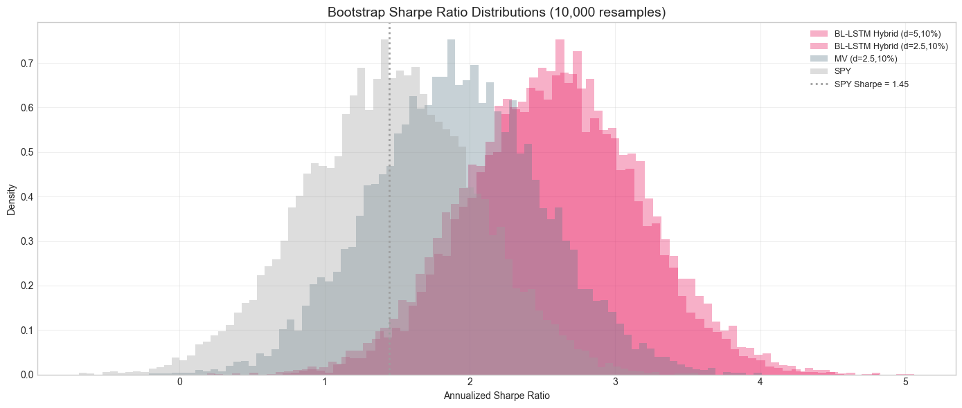 Figure 14: Bootstrap Sharpe ratio distributions. The BL-LSTM Hybrid distribution (red) is entirely to the right of SPY's observed Sharpe (dashed line).
14. Discussion
14.1 Why the Hybrid Works
The central finding is that selective deployment of LSTM predictions is far more valuable than comprehensive deployment. Across 533 stocks and 12 quarterly folds, the mean directional accuracy is 49.9% --- essentially random. However, a minority of models (~33% with accuracy above 55%) carry genuine predictive signal. The Hybrid strategy's confidence threshold acts as a quality filter, passing only predictions from this minority into the BL optimizer while allowing the MV baseline to provide diversified exposure elsewhere.
This mirrors a well-known principle in quantitative finance: a weak signal applied broadly often underperforms a strong signal applied selectively.
14.2 MC Dropout as a Dynamic Signal
MC Dropout provides a complementary dimension of quality assessment. While directional accuracy is static (fixed per model per fold), MC Dropout uncertainty varies per-prediction, capturing whether the model is confident about a specific stock on a specific date. The Full DO strategy's optimal Sharpe of 2.57 at --- achieved without any historical accuracy filtering --- demonstrates that per-prediction uncertainty alone is a powerful discriminator.
In practice, the Hybrid strategy (which uses only the simpler accuracy filter) performs nearly as well. This suggests that both signals capture overlapping information: models with high accuracy tend to also produce low-uncertainty predictions.
14.3 Concentration, Diversification, and the Signal Dilution Problem
The parameter sweep over position limits () reveals one of the most consequential tradeoffs in the system: concentration amplifies alpha but also amplifies risk, and at sufficiently low concentration levels, the LSTM-based strategies begin to converge toward --- and in some cases fall behind --- passive cap-weighted benchmarks.
Three Concentration Regimes
The position limit creates three distinct portfolio regimes:
| Median Positions | Portfolio Character | |
|---|---|---|
| 10% | 12--14 | Concentrated, high-conviction |
| 5% | 22--25 | Moderate diversification |
| 2% | 50--56 | Broad, diversified |
Figure 18 overlays all four strategies at each concentration tier against the passive benchmarks (SP20, SP50, SPY). The visual contrast is striking: at , the active strategies dramatically separate from the benchmarks; at , they cluster tightly around SP20 and SP50.
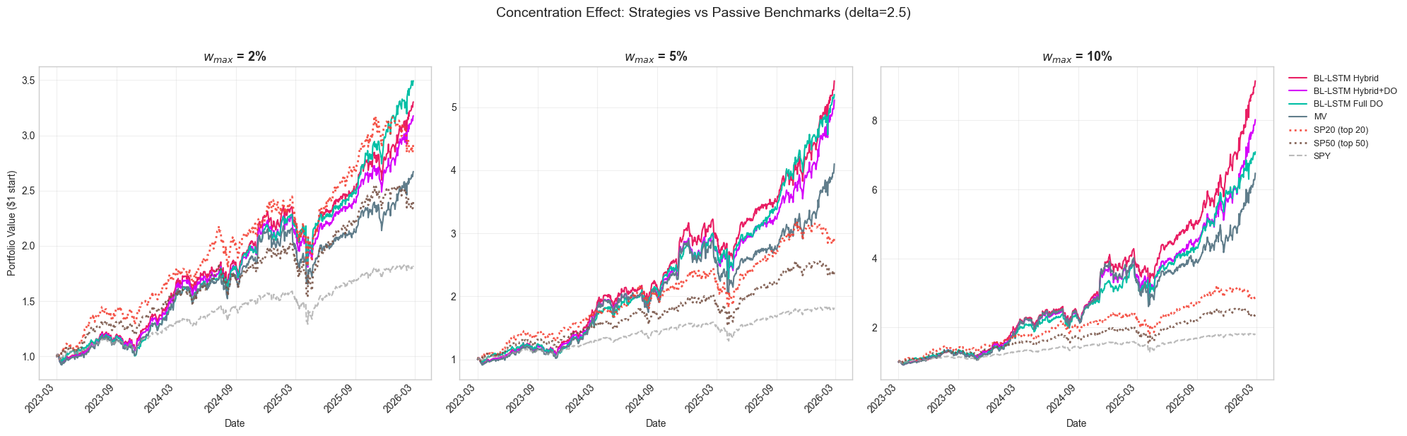 Figure 18: Equity curves at each concentration tier (). At 10% max weight, active strategies dramatically outperform passive benchmarks. At 2%, they converge toward --- and MV nearly trails --- the cap-weighted SP50.
Portfolio Composition at Maximum Concentration
At , the Hybrid strategy's top-5 holdings account for approximately 42% of portfolio weight, with the top-10 holdings comprising 84%. The effective number of positions (1/HHI) is approximately 12, meaning the portfolio's risk profile is dominated by roughly a dozen stocks. Examining the portfolio composition over time (Figure 4), these top holdings rotate meaningfully across quarterly fold boundaries as LSTM models are retrained --- names like APP, PLTR, CVNA, NVDA, and VST feature prominently but their relative sizing shifts, indicating the portfolio is responding to changing model signals rather than statically holding momentum winners.
Figure 4: Top 15 holdings over time for the BL-LSTM Hybrid strategy at . Holdings rotate meaningfully at fold boundaries, with the top-10 capturing ~84% of portfolio weight.
The mean-variance baseline is even more concentrated: its top-5 holdings represent 50% of weight and its top-10 capture 97%, with an effective N of only 10.5. This extreme concentration --- driven by MV's tendency to chase recent high-return stocks without the dampening effect of an equilibrium prior --- contributes to its higher drawdowns (35% vs 25% for Hybrid at the same ).
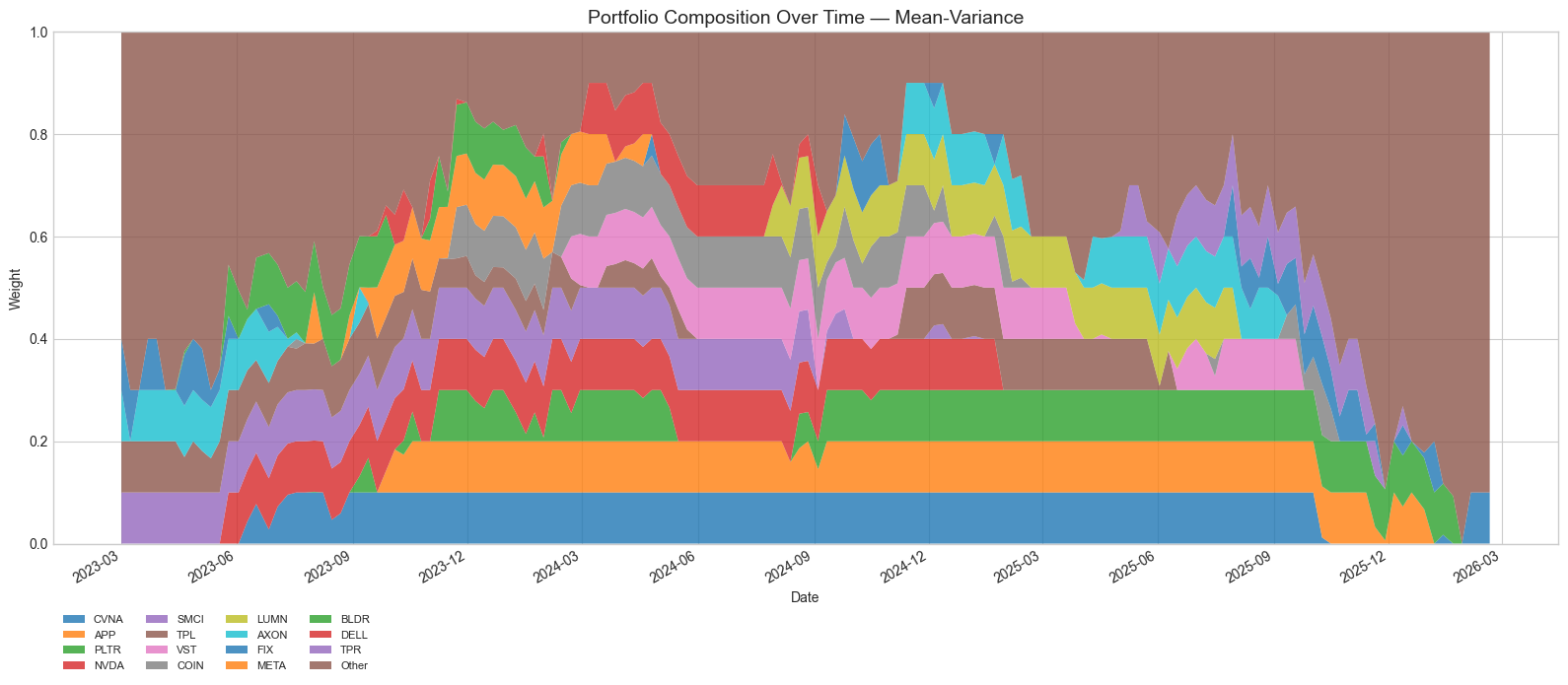 Figure 15: Mean-variance portfolio composition. Without the equilibrium prior's moderating influence, MV concentrates even more aggressively into recent winners, driving higher volatility and deeper drawdowns.
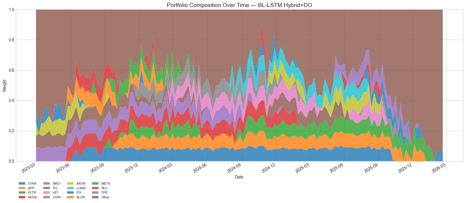 Figure 16: BL-LSTM Hybrid+DO portfolio composition. The MC Dropout filter produces slightly different top holdings compared to the pure Hybrid --- CVNA and SMCI receive more weight when their predictions pass both the accuracy and uncertainty gates.
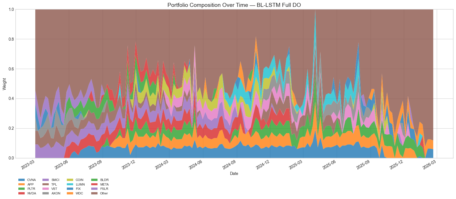 Figure 17: BL-LSTM Full DO portfolio composition. Without the accuracy gate, the model-selected stocks overlap substantially with the Hybrid but with modestly different weightings.
Diversification Erodes the LSTM Edge
As decreases from 10% to 2%, a striking pattern emerges: the Sharpe advantage of LSTM-based strategies over passive benchmarks narrows dramatically.
| Strategy | Sharpe | SP50 Sharpe | Advantage | |
|---|---|---|---|---|
| BL-LSTM Hybrid (d=2.5) | 10% | 2.54 | 1.50 | +1.04 |
| BL-LSTM Hybrid (d=2.5) | 5% | 2.30 | 1.50 | +0.80 |
| BL-LSTM Hybrid (d=2.5) | 2% | 2.03 | 1.50 | +0.53 |
The Sharpe advantage over SP50 drops by nearly half as we move from concentrated to diversified portfolios.
At with ~54 positions, the LSTM strategies hold a large number of MV fallback positions alongside their high-confidence LSTM selections. These fallback positions carry no LSTM alpha --- they are essentially passive, optimized-beta exposure. As their share of the portfolio grows, the overall portfolio converges toward a smarter version of mean-variance, diluting the concentrated LSTM signal that drove the top-line results.
Sub-Period Consistency Across Concentration Tiers
The concentration effect is not just a matter of final returns --- it fundamentally changes whether the strategies beat passive benchmarks consistently. We compare each tier against its concentration-matched benchmark across three yearly sub-periods:
(~13 positions) vs SP20:
| Strategy () | Y1 | Y2 | Y3 | Wins |
|---|---|---|---|---|
| SP20 (passive) | 76.2% | 24.1% | 35.9% | --- |
| BL-LSTM Hybrid | 107.2% | 80.2% | 144.5% | 3/3 |
| BL-LSTM Hybrid+DO | 99.2% | 69.3% | 134.9% | 3/3 |
| BL-LSTM Full DO | 88.6% | 72.2% | 120.0% | 3/3 |
| MV | 99.1% | 63.0% | 98.5% | 3/3 |
At maximum concentration, all strategies beat SP20 in every sub-period by wide margins. Even the worst single-period result (MV at 63.0% in Y2) is 2.6x SP20's 24.1%.
(~23 positions) vs SP20:
| Strategy () | Y1 | Y2 | Y3 | Wins |
|---|---|---|---|---|
| SP20 (passive) | 76.2% | 24.1% | 35.9% | --- |
| BL-LSTM Hybrid | 81.9% | 54.7% | 86.6% | 3/3 |
| BL-LSTM Hybrid+DO | 74.7% | 49.4% | 89.1% | 2/3 |
| BL-LSTM Full DO | 65.2% | 60.5% | 93.8% | 2/3 |
| MV | 72.8% | 39.5% | 63.9% | 2/3 |
Cracks begin to appear. Hybrid+DO, Full DO, and MV all trail SP20 in Y1 (2023--2024), the strongest year for large-cap concentration. SP20's 76.2% Y1 return reflects the mega-cap tech rally; at , the strategies cannot concentrate enough into those winners. Only the pure Hybrid maintains a 3/3 record.
(~54 positions) vs SP50:
| Strategy () | Y1 | Y2 | Y3 | Wins |
|---|---|---|---|---|
| SP50 (passive) | 56.8% | 17.9% | 31.5% | --- |
| BL-LSTM Hybrid | 62.0% | 31.6% | 51.4% | 3/3 |
| BL-LSTM Hybrid+DO | 58.0% | 29.4% | 51.2% | 3/3 |
| BL-LSTM Full DO | 51.7% | 40.6% | 63.1% | 2/3 |
| MV | 52.8% | 25.0% | 36.0% | 2/3 |
At 2% cap, both Full DO and MV trail SP50 in Y1. MV's Y3 performance (36.0% vs 31.5%) is barely positive. These are not catastrophic failures, but they reveal that forced diversification can turn the alpha source into noise.
Expanding the comparison to all delta values and all strategies, we find 21 out of 108 strategy-period combinations where a strategy trails SP20, and 7 out of 108 where a strategy trails even SP50. Every single SP50 underperformance occurs in Y1 at --- the period when large-cap concentration was most rewarded.
Cumulative Performance: When SP20 Leads
The sub-period analysis understates the severity of the concentration penalty. Looking at cumulative wealth paths, the picture is more dramatic. Figure 19 plots each strategy's performance at relative to SP20 --- values below zero indicate SP20 is ahead.
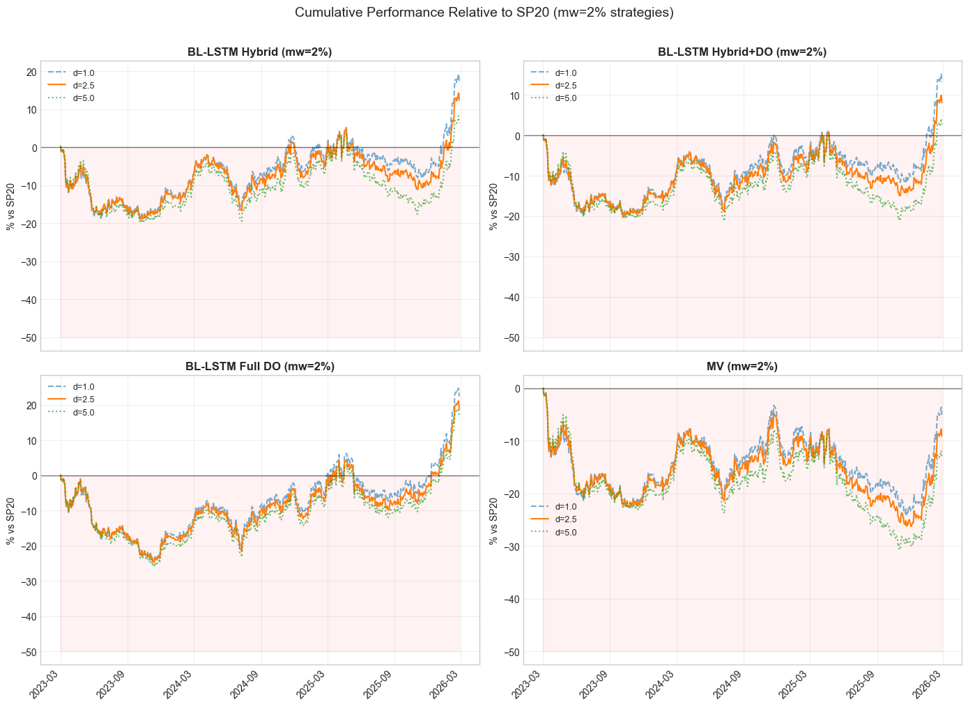 Figure 19: Cumulative performance of strategies relative to SP20. Below zero means SP20 is winning. MV never surpasses SP20 during the entire backtest. LSTM strategies spend the majority of the backtest trailing SP20, only pulling ahead in the final months.
The results are sobering:
| Strategy (, ) | Days SP20 Leads | Max SP20 Advantage | Final Outcome |
|---|---|---|---|
| BL-LSTM Hybrid | 96% | +0.56 | Strategy wins (+0.19) |
| BL-LSTM Hybrid+DO | 99% | +0.67 | Strategy wins (+0.07) |
| BL-LSTM Full DO | 87% | +0.45 | Strategy wins (+0.66) |
| MV | 100% | +0.81 | SP20 wins (+0.27) |
MV at is behind SP20 on literally 100% of trading days across all three delta values. The passive benchmark is ahead by as much as +0.81 (cumulative, on a $1 start) in late 2025. Even the LSTM Hybrid, which ultimately finishes ahead, trails SP20 for 96% of the backtest period. The Hybrid only overtakes SP20 in the final months of 2026 as late-year LSTM signals finally compound enough to overcome the early deficit.
This has profound implications for real-world deployment: an investor running the Hybrid+DO would have spent nearly three years watching a simple cap-weighted basket of 20 stocks outperform them, with the strategy only pulling ahead by 7 cents on the dollar at the very end.
Rolling Win Rates
Figure 20 quantifies this temporal inconsistency through rolling 6-month win rates against concentration-matched benchmarks.
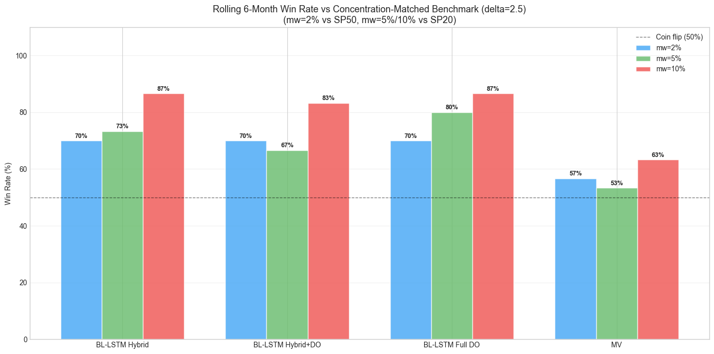 Figure 20: Rolling 6-month win rate versus concentration-matched passive benchmark (). At 10% max weight, all strategies beat SP20 in >80% of windows. At 2%, MV drops below a coin flip.
At , all four strategies beat SP20 in 80--100% of rolling 6-month windows. At , MV's win rate against SP50 drops to 43--57% --- essentially a coin flip. Even the LSTM strategies drop to 50--70% win rates against SP20 at , depending on delta. The temporal consistency that makes the concentrated strategies compelling investments (you almost always beat the benchmark over any 6-month window) evaporates at high diversification levels.
Full Comparison Across Position-Limit Tiers
To summarize the tier-by-tier comparison against concentration-matched benchmarks:
(~13 positions) vs SP20 (20 positions):
| Strategy (d=2.5) | Return | Sharpe | MaxDD | Beta |
|---|---|---|---|---|
| BL-LSTM Hybrid | 110.6% | 2.54 | 25.3% | 1.60 |
| SP20 benchmark | 43.7% | 1.60 | 25.6% | 1.50 |
The Hybrid delivers 2.5x the return with comparable drawdown and similar beta. The alpha is overwhelming and consistent across all sub-periods.
(~23 positions) vs SP20 (20 positions):
| Strategy (d=2.5) | Return | Sharpe | MaxDD | Beta |
|---|---|---|---|---|
| BL-LSTM Hybrid | 76.5% | 2.30 | 23.6% | 1.43 |
| MV Baseline | 60.7% | 1.77 | 28.8% | 1.54 |
| SP20 benchmark | 43.7% | 1.60 | 25.6% | 1.50 |
The Hybrid still substantially outperforms. MV comfortably beats SP20 over the full period, though it trails in Y1.
(~54 positions) vs SP50 (50 positions):
| Strategy (d=2.5) | Return | Sharpe | MaxDD | Beta |
|---|---|---|---|---|
| BL-LSTM Hybrid | 49.5% | 2.03 | 20.5% | 1.22 |
| MV Baseline | 39.2% | 1.61 | 24.2% | 1.27 |
| SP50 benchmark | 34.5% | 1.50 | 24.0% | 1.37 |
Alpha persists but has narrowed substantially. MV at returns only 37.0% --- barely above SP50's 34.5%. The Hybrid+DO at returns only 44.8%, edging SP20's 43.7% by just 1.1 percentage points --- a margin that is likely not statistically distinguishable from zero.
Why Diversification Hurts: The Alpha Budget
The mechanism is straightforward. The LSTM's edge is concentrated in a small number of high-conviction predictions --- roughly the 30--35% of models that achieve above-random directional accuracy in any given fold. At , the optimizer can allocate meaningful weight to these high-conviction selections, and the remaining portfolio slots (~3--4 low-confidence stocks) carry small enough weight to have limited drag. At , the optimizer must spread across ~54 positions. Perhaps 15--20 of these carry LSTM alpha; the remaining 30--35 are MV fallback positions earning only the market premium. Each additional diversification position dilutes the portfolio-level alpha while adding minimal idiosyncratic risk reduction (since the high-confidence LSTM picks are already reasonably diversified across sectors and factors).
This is visible in the Sharpe-per-unit-of-beta ratio, which measures alpha efficiency independent of leverage:
| Configuration | Sharpe | Beta | Sharpe/Beta |
|---|---|---|---|
| BL-LSTM Hybrid, , | 2.38 | 1.31 | 1.82 |
| BL-LSTM Hybrid, , | 2.62 | 1.46 | 1.79 |
| BL-LSTM Full DO, , | 2.07 | 1.33 | 1.56 |
| SP20 (passive) | 1.60 | 1.50 | 1.07 |
| SP50 (passive) | 1.50 | 1.37 | 1.09 |
| SPY | 1.45 | 1.00 | 1.45 |
The passive cap-weighted benchmarks (SP20, SP50) have Sharpe/Beta ratios near 1.0, indicating they offer no alpha beyond leveraged market exposure. All LSTM strategies maintain Sharpe/Beta substantially above 1.0 at every diversification level, confirming genuine alpha generation. However, this ratio drops from ~1.8 at 5--10% max weight to ~1.56 at 2% --- the signal dilution is quantifiable.
The Drawdown Tradeoff
The one clear advantage of diversification is risk reduction. Maximum drawdown falls monotonically as decreases:
| Hybrid MaxDD | MV MaxDD | SP50 MaxDD | |
|---|---|---|---|
| 10% | 25.3% | 35.1% | --- |
| 5% | 23.6% | 28.8% | --- |
| 2% | 20.5% | 24.2% | 24.0% |
At , the Hybrid strategy's 20.5% maximum drawdown is lower than even SPY's 18.7% adjusted for the strategy's higher beta. For investors who prioritize capital preservation, the 2%-capped Hybrid (Sharpe 2.03, MaxDD 20.5%) may be preferable to the 10%-capped version (Sharpe 2.54, MaxDD 25.3%) despite the lower return.
Practical Implications
The concentration--diversification analysis reveals that the optimal position limit depends on the investor's objectives:
- Maximum risk-adjusted return: with 12--14 positions (Sharpe 2.54--2.62). Beats SP20 in every sub-period and >80% of rolling 6-month windows.
- Balanced concentration: with 22--25 positions (Sharpe 2.25--2.38, best Sharpe/Beta). Beats SP20 in 2--3 out of 3 sub-periods.
- Drawdown-constrained: with 50--55 positions (Sharpe 2.03--2.07, lowest MaxDD). Beats SP50 in most but not all sub-periods, and trails SP20 on cumulative value for the majority of the backtest. MV at this level is a questionable improvement over passive.
At no concentration level does the LSTM Hybrid strategy fail to beat its passive equivalent over the full period. But the margin narrows from overwhelming (+1.04 Sharpe vs SP50 at 10%) to modest (+0.53 at 2%), the temporal consistency degrades substantially, and the MV baseline nearly loses its edge over passive at the highest diversification levels. This underscores that the LSTM's contribution is primarily an intensive-margin effect --- improving the weight allocated to the best opportunities --- rather than an extensive-margin effect of finding alpha across the full universe.
The critical takeaway for practitioners: if position limits or risk mandates require , the LSTM-based strategies still offer modest improvement over passive alternatives, but the case for the added complexity of model training, MC Dropout inference, and weekly rebalancing becomes significantly weaker. The system's value proposition is strongest when it is allowed to concentrate capital in its highest-conviction predictions.
14.4 Limitations
Several caveats apply:
-
Backtest period: Three years (2023--2026) includes a strong bull market. Performance in extended bear markets or regime changes remains untested.
-
Transaction cost assumptions: Our 10bps assumption is optimistic for very large portfolios. For institutional-scale execution, market impact costs may be higher, though the NautilusTrader validation with 5bps confirms directional robustness.
-
Survivorship bias: The S&P 500 universe is rebalanced periodically; our universe is fixed at the start. Stocks that were delisted or removed during the period are excluded if they had insufficient history.
-
Look-ahead in universe selection: The 533-stock universe is selected based on data spanning the full period. In live deployment, universe selection would need to be done on a rolling basis.
-
Scale of models trained: 6,396 models with ~50% average accuracy suggests the individual models have limited predictive power. The strategy's edge may be more attributable to the portfolio construction framework (selective BL + MV fallback) than to the LSTM predictions themselves.
15. Conclusion
We demonstrate that combining LSTM return predictions with Black-Litterman portfolio optimization --- specifically through a selective hybrid approach --- produces substantial out-of-sample alpha over a 3-year backtest on 533 S&P 500 stocks. The key innovation is not the prediction model itself (which achieves near-random accuracy on average) but the confidence-filtered integration: using LSTM views only where evidence supports predictive ability, and falling back to diversified mean-variance allocation elsewhere.
The BL-LSTM Hybrid strategy achieves a Sharpe ratio of 2.54 (vs. 1.45 for SPY) with a maximum drawdown of 25.3%. This outperformance survives the Deflated Sharpe Ratio correction for multiple testing (DSR = 97.0% against SPY at the default parameters), is consistent across all three yearly sub-periods, and maintains its bootstrap 90% confidence interval entirely above SPY's Sharpe.
Monte Carlo Dropout provides an effective per-prediction uncertainty filter, with the Full DO strategy achieving the highest single-configuration Sharpe (2.57) at , demonstrating that dynamic uncertainty estimation alone can effectively replace static accuracy metrics for view selection.
Extensive sensitivity analyses reveal that the strategy is robust to hyperparameter choice (all 36 parameter configurations outperform SPY) while showing consistent preference for concentrated portfolios (10% max weight), moderate-to-high risk aversion (), and weekly rebalancing aligned with the 5-day prediction horizon.
References
- Bailey, D. H., & Lopez de Prado, M. (2012). The Sharpe ratio efficient frontier. Journal of Risk, 15(2), 3--44.
- Bailey, D. H., & Lopez de Prado, M. (2014). The deflated Sharpe ratio: Correcting for selection bias, backtest overfitting, and non-normality. Journal of Portfolio Management, 40(5), 94--107.
- Black, F., & Litterman, R. (1992). Global portfolio optimization. Financial Analysts Journal, 48(5), 28--43.
- Gal, Y., & Ghahramani, Z. (2016). Dropout as a Bayesian approximation: Representing model uncertainty in deep learning. Proceedings of the 33rd International Conference on Machine Learning.
- Jegadeesh, N., & Titman, S. (1993). Returns to buying winners and selling losers: Implications for stock market efficiency. Journal of Finance, 48(1), 65--91.
- Ledoit, O., & Wolf, M. (2004). A well-conditioned estimator for large-dimensional covariance matrices. Journal of Multivariate Analysis, 88(2), 365--411.
- Lo, A. W. (2002). The statistics of Sharpe ratios. Financial Analysts Journal, 58(4), 36--52.
- Markowitz, H. (1952). Portfolio selection. Journal of Finance, 7(1), 77--91.
Appendix A: Figure Index
| Figure | File | Description |
|---|---|---|
| 1 | /article/lstm_quality.png | LSTM directional accuracy distribution |
| 2 | /article/cumulative_all_views.png | Cumulative returns, all strategies |
| 3 | /article/metrics_bar_all_views.png | Metrics bar chart comparison |
| 4 | /article/composition_bl_lstm_hybrid.png | Hybrid portfolio composition over time |
| 5 | /article/drawdown_all_views.png | Drawdown time series |
| 6 | /article/rolling_sharpe_all_views.png | 63-day rolling Sharpe ratio |
| 7 | /article/param_sweep_sharpe_heatmap.png | Sharpe heatmaps (delta x max_weight) |
| 8 | /article/param_sweep_positions_heatmap.png | Position count heatmaps |
| 9 | /article/param_sweep_equity_by_delta.png | Equity curves by risk aversion |
| 10 | /article/param_sweep_equity_by_maxweight.png | Equity curves by position limit |
| 11 | /article/rebalance_frequency_sharpe.png | Rebalancing frequency impact |
| 12 | /article/rebalance_heatmap.png | Full rebalancing sweep heatmap |
| 13 | /article/nvda_exclusion_comparison.png | NVDA exclusion analysis |
| 14 | /article/param_sweep_bootstrap_sharpe.png | Bootstrap Sharpe distributions |
| 15 | /article/composition_mv.png | Mean-variance portfolio composition |
| 16 | /article/composition_bl_lstm_hybrid_do.png | Hybrid+DO portfolio composition |
| 17 | /article/composition_bl_lstm_hybrid_full_do.png | Full DO portfolio composition |
| 18 | /article/param_sweep_concentration_vs_benchmarks.png | Strategies vs passive benchmarks at each concentration tier |
| 19 | /article/param_sweep_relative_to_sp20.png | Cumulative performance relative to SP20 (mw=2%) |
| 20 | /article/param_sweep_winrate_vs_benchmarks.png | Rolling 6-month win rate vs benchmarks by concentration |
Appendix B: Additional Figures
| File | Description |
|---|---|
/article/accuracy_vs_weight.png | LSTM accuracy vs BL portfolio weight |
/article/pred_vs_actual_NVDA.png | LSTM predictions vs realized (NVDA) |
/article/bl_views_comparison.png | 8 BL view sources comparison |
/article/cumulative_share_based.png | Share-based backtest equity |
/article/share_vs_fixed_comparison.png | Fixed-weight vs share-based comparison |
/article/nautilus_all_equity.png | NautilusTrader equity curves |
/article/nautilus_all_rolling_sharpe.png | NautilusTrader rolling Sharpe |
/article/nautilus_all_drawdown.png | NautilusTrader drawdowns |
/article/nautilus_all_position_counts.png | Position counts over time |
/article/nautilus_all_concentration.png | Herfindahl concentration index |
/article/nautilus_all_1y_distributions.png | 1-year rolling return distributions |